Open Shortest Path First (OSPF) is the first link-state protocol that you will learn about. Apart from being a link-state protocol, it is also an open standard protocol. What this means is that you can run OSPF in a network consisting of multivendor devices. You may have realized that you cannot run EIGRP in a network that consists of non-Cisco devices. This makes OSPF a very important protocol to learn.
Compared to EIGRP, OSPF is a more complex protocol and supports all features such as VLSM/CIDR and more. A brief summary of OSPF features is given below:
- Works on the concept of Areas and Autonomous systems
- Highly Scalable
- Supports VLSM/CIDR and dis-contiguous networks
- Does not have a hop count limit
- Works in multivendor environment
- Minimizes updates between neighbors.
While the above list is a very basic overview of the features of OSPF and will be expanded on in coming sections, it is a good time to take a step back and compare the four protocols detailed in this chapter. Table 5-2 shows a comparison of the four protocols.
Table 5-2 Comparison of routing protocols.
| Features | OSPF | EIGRP | RIPv1 | RIPv2 |
| Protocol Type | Link state | Hybrid | Distance Vector | Distance Vector |
| Classful Protocol | No | No | Yes | No |
| VLSM Support | Yes | Yes | No | Yes |
| Discontiguous Network Support | Yes | Yes | No | Yes |
| Hop count limit | None | 255 | 15 | 15 |
| Routing Updates | Event Triggered | Event Triggered | Periodic | Periodic |
| Complete Routing table shared | During new adjacencies | During new adjacencies | Periodic | Periodic |
| Mechanism for sharing updates | Multicast | Multicast and unicast | Multicast | Broadcast |
| Best Path computation | Dijkstra | DUAL | Bellman-Form | Bellman-Ford |
| Metric used | Bandwidth | Bandwidth and Delay (default) | Hop Count | Hop Count |
| Organization type | Hierarchical | Flat | Flat | Flat |
| Convergence | Fast | Very Fast | Slow | Slow |
| Auto Summarization | No | Yes | Yes | Yes |
| Manual Summarization | Yes | Yes | No | No |
| Peer authentication | Yes | Yes | Yes | No |
It should be noted here that OSPF has many more features that the ones listed in Table 5-2 and than those covered in this book. One feature that really separates OSPF from other protocols is its support of a hierarchical design. What this means is that you can divide a large internetwork into smaller internetworks called areas. It should be noted that these areas, though separate, still lie within a single OSPF autonomous system. This is distinctly different from the way EIGRP can be divided into multiple autonomous systems. While in EIGRP each autonomous system functions independent of others and a redistribution is required to share routes, in OSPF areas are dependent on each other and routes are shared between them without redistribution.
You should also know that like EIGRP, OSPF could be divided into multiple Autonomous Systems. Each autonomous system will be different from the rest and will require redistribution of routes.
The hierarchical design of OSPF provides the following benefits:
- Decrease routing overhead and flow of updates
- Limit network problems such as instability to an area
- Speed up convergence.
One disadvantage of this is that planning and configuring OSPF is more difficult than other protocols. Figure 5-5 shows a simple OSPF hierarchical setup. In the figure notice that Area 0 is the central area and the other two areas connect to it.
Figure 5-5 OSPF hierarchical design
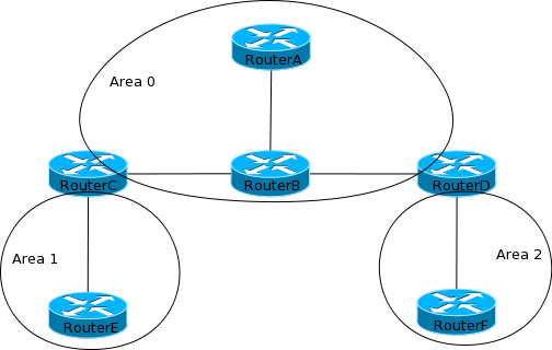
This is always true in an OSPF design. All areas need to connect to Area 0. Areas that cannot connect to area 0 physically need a logical connection it using something known as virtual links. Virtual links are out of the scope of the CCNA exam.
Another important thing to notice in the figure is that for each area, there is a router that connects to area 0 as well. These routers are called Area Border Routers (ABRs). In Figure 5-5, RouterC and RouterD are ABRs because they connect to area 0 as well as another area. The way ABRs connect different areas, routers that connect different autonomous systems are called Autonomous System Boundary Routers (ASBRs). In Figure 5-5, if RouterE connect to another OSPF AS or to an AS of another protocol such as EIGRP, it would be called an ASBR.
From Figure 5-5, you learned about three OSPF terms – Area, ABR and ASBR. Similarly there are many other terms associated with OSPF that you need to be aware of before getting into how OSPF actually works. The next section looks at some of these terms.
Building Blocks of OSPF
Each routing protocol has its own language and terminologies. In OSPF there are various terms that you should be aware of. This section looks at the some of the important terminologies associated with OSPF. In an attempt to make it easier to understand and remember, the terminologies are broken into three parts here – Router level, Area level and Internetwork level.
At the Router level, when OSPF is enabled, it becomes aware of the following first:
- Router ID – Router ID is the IP address that will represent the router throughout the OSPF AS. Since a router may have multiple IP addresses (for its multiple interfaces), Cisco routers choose the highest loopback interface IP address. (Do not worry if you do not know what loopback interfaces are. They are covered later in the chapter). If loopback interfaces are not present, OSPF chooses the highest physical IP address configured within the active interfaces. Here highest literally means higher in number (Class C will be higher than Class A because 192 is greater than 10).
- Links – Simply speaking a Link is a network to which a router interface belongs. When you define the networks that OSPF will advertise, it will match interface addresses that belong to those networks. Each interface that matches is called a link. Each link has a status (up or down) and an IP address associated with it.
Let’s take a simple test here. Look at Figure 5-6 and try to find the Router ID and links on each of the routers.
Figure 5-6 RouterID and links
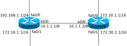
For RouterA, the RouterID will be 192.168.1.1 because it is the highest physical IP address present. The three links present on RouterA are the networks 192.168.1.0/24, 10.0.0.0/8 and 172.16.0.0/16. Similarly, the Router ID of RouterB is 172.30.1.1 since that is the highest physical IP address on the router. The three links present on RouterB are 10.0.0.0/8, 172.20.0.0/16 and 172.30.0.0/16.
Once a router is aware of the above two things, it will try to find more about its network by seeking out other OSPF speaking routers. At that stage the following terms come into use:
- Hello Packets – Similar to EIGRP hello packets, OSPF uses hello packets to discover neighbors and maintain relationships. Hello packet contains information such as area number that should match for a neighbor relation to be established. Hello packets are sent to multicast address 224.0.0.5.
- Neighbors – Neighbors is the term used to define two or more OSPF speaking routers connected to the same network and configured to be in the same OSPF area. Routers use hello packets to discover neighbors.
- Neighbor Table – OSPF will maintain a list of all neighbors from which hello packets have been received. For each neighbor various details such as RouterID and adjacency state are stored.
- Area – An OSPF area is a grouping of networks and routers. Every router in the area shares the same area id. Routers can belong to multiple areas; therefore, area id is linked to every interface. Routers will not exchange routing updates with routers belonging to different areas. Area 0 is called the backbone area and all other area must connect to it by having at least one router that belongs to both areas.
Once OSPF has discovered neighbors it will look at the network type on which it is working. OSPF classifies networks into the following types:
- Broadcast (multi-access) – Broadcast (multi-access) networks are those that allow multiple devices to access (or connect to) the same network and also provide ability to broadcast. You will remember that when a packet is destined to all devices in a network, it is termed as a broadcast. Ethernet is an example of a broadcast multi-access network.
- Non-Broadcast multi-access (NBMA) – Networks that allow multi-access but do not have broadcast ability are called NBMA networks. Frame Relay networks are usually NBMA.
- Point-to-Point – Point-to-Point networks consist of direct connection between two routers and provide a single path of communication. When routers are connected back-to-back using serial interfaces, a point-to-point network is created. Point-to-point networks can also exist logically across geographical locations using various WAN technologies such as Frame Relay and PPP.
- Point-to-Multipoint – Point-to-Multipoint networks consist of multiple connections between a single interface of a router and multiple remote routers. All routers belong to the same network but have to communicate via the central router, whose interface connects the remote routers.
Depending on the network type that OSPF discovers on the router interfaces, it will need to form Adjacencies. An adjacency is the relation between neighbors that allows direct exchange of routes. Unlike EIGRP, OSPF will not form adjacency with all neighbors always. A router will form adjacencies with a few or all neighbors depending on the network type that is discovered. Adjacencies in each network type is discussed below:
- Broadcast (multi-access) – Since multiple routers can connect to such networks, OSPF elects a Designated Router (DR) and a Backup Designated Router (BDR). All routers in these networks, form adjacencies only with the DR and BDR. This also means that route updates are only shared between the routers and the DR and BDR. It is the duty of the DR to share routing updates with the rest of the routers in the network. If a DR loses connectivity to the network, the BDR will take its place. The election process is discussed later in the chapter.
- NBMA – Since NBMA is also a multi-access network, a DR and a BDR is elected and routers form adjacencies only with them. The problem with NBMA networks is that since broadcast capability and in turn multicast capability is not present, routers cannot discover neighbors. So NBMA networks require you to manually tell OSPF about the neighbors present in the network. Apart from this, OSPF functions as it does in a broadcast multi-access network.
- Point-to-Point – Since there are only two routers present in a point-to-point network, there is no need to elect a DR and BDR. Both routers form adjacency with each other and exchange routing updates. Neighbors are discovered automatically in these networks.
- Point-to-multipoint – Point-to-multipoint interfaces are treat as special point-to-point interfaces by OSPF and it does a little extra work on here that is out of scope of CCNA. There is no DR/BDR election in such networks and neighbors are automatically discovered.

Once OSPF has formed adjacencies, it will start exchanging routing updates. The following two terms come to use here:
- Link State Advertisements – Link State Advertisements (LSAs) are OSPF packets containing link-state and routing information. These are exchanged between routers that have formed adjacencies. The packets essentially tell routers in the networks about different networks (links) that are present and how to reach them. Different types of LSAs are discussed later in the chapter.
- Topology Table – The topology table contains information on every link the router learns about (via LSAs). The information is the topology table is used to compute the best path to remote networks.
At the area level, the only term that gets introduced is:
- Area Border Routers (ABRs) – Routers that connect an area to area 0 are called ABRs. They have one interface belonging to area 0 and other interfaces belonging to one or more areas. They are responsible for propagating routing updates between area 0 and other areas.
At the internetwork level another term that gets introduced is:
- Autonomous System Boundary Router (ASBR) – A router that connects an OSPF AS to another OSPF AS or AS belonging to other routing protocols is called an Autonomous System Boundary Router or ASBR. Route redistribution is setup between the two AS on these routers and hence they become the gateway between the two AS.
Now that you are familiar with OSPF terminology, the rest of the sections will discuss the working of OSPF in detail and help you better understand the terms discussed here.
Loopback Interfaces
Loopback interfaces are virtual, logical interfaces that exist in the software only. They are used for administrative purposes such as providing a stable OSPF interface or diagnostics. Using loopback interfaces with OSPF has the following benefits:
- Provides an interface that is always active.
- Provides an OSPF Router ID that is predictable and always same. Making is easier to troubleshoot OSPF.
- Router ID is a differentiator in DR/BDR election. Having a loopback interface with higher order IP address can influence the election.
Configuring a loopback interface is easy – You need to select an interface number and enter the interface configuration mode using the interface command in global configuration mode as shown below:
RouterA(config-if)#
The interface number can be any number starting from 0. Once in the interface configuration mode, use the ip address command to configure an IP address as you would on a physical interface. An example is shown below:
That’s it! The loopback interface is configured and will be listed as an active interface in the show ip interface command.
The loopback interface can be important for OSPF because it will take the highest loopback IP address as the Router ID. If a loopback interface is not present, the highest physical IP address will be taken.
A loopback interface is logically equivalent to a physical address. The router is going to add an entry into its routing table for the network that the loopback interface address belongs to. So you can even configure a routing protocol to advertise the loopback network. Whether you choose to do that or not depends on whether you want the loopback address to be reachable from the network or not. Remember you will be using a subnet if you decide to advertise the loopback network.
DR/BDR Election and influencing it
As discussed earlier, in multi-access network types, DRs and BDRs are elected and routers in the area only form adjacencies with them. So DRs and BDRs are an important part of OSPF and usually determine how well OSPF will function. In this section you will learn about the process by which DRs/BDRs are elected. Before learning about the process, it is important that you understand the terms neighbors and adjacencies fully since they are central to functioning of OSPF and the election process.
A router running OSPF will periodically send out Hello packets to multicast address 224.0.0.5. These hello packets serve as a way to discover neighbors. When a router receives these packets, it checks the following to ascertain that a neighborship can be established:
- Area ID – The Area ID received in a hello packet should match the area ID associated with the interface the packet was received on. As mentioned earlier, OSPF associates an area ID with each interface it is enabled on. The rationale behind comparing the area ID is that only router having interface in the same area should form neighborship.
- Hello and Dead intervals – Hello packets exchanged by routers running OSPF contain information such as area ID, hello interval and dead interval. Hello interval specifies the time duration between hello packets and dead interval specifies the time duration after which a router will be declared dead if hello packets have not been received from it.
For a neighborship to form, the hello and dead intervals should match between the routers.
- Authentication – OSPF allows you to set a password for an area. For neighborship to form, the password must be same on the routers. Setting a password is optional.
If all the three above conditions match, the router will add the neighbor into the neighbor table and form a neighborship. Even though a neighborship gets formed, OSPF unlike EIGRP will not share routing updates, or link state advertisements in this case, with every neighbor.
For OSPF to share link state advertisements, an adjacency must be formed between the routers. As discussed earlier, how adjacencies are formed depends on the network type. In a multi-access network, a DR and BDR will be elected and all routers in the network will form adjacency with them only. Each router will exchange LSAs with DR and BDR. DR in turn will relay the information to the rest of the routers.
When routers realize that they are connected to a multi-access network, they will look at each Hello packet received to find the priority and Router ID of each router. Then the priority is compared and the router with the highest priority is selected the DR. The router with the second highest priority becomes the BDR. By default the priority of each router is 1 and can be changed on a per-interface basis.
If all routers have the default priority, then the router with the highest Router ID is elected the DR while the router with the second highest Router ID is elected the BDR. If the priority of a router is set to zero, it will not participate in the election process and will never be a DR or BDR.
As you know, the Router ID is the highest physical IP address present on a Router. This can be overridden by using a loopback interface because a router will use the highest loopback address, if one is present.
If you need to influence the DR/BDR election in a network segment, you can do one of the following:
- Manually increase the priority of a router interface to ensure that the router becomes the DR/BDR.
- Configure a loopback interface so that the Router ID becomes higher than that of the other routers in the network segment.
SPF Tree Calculation
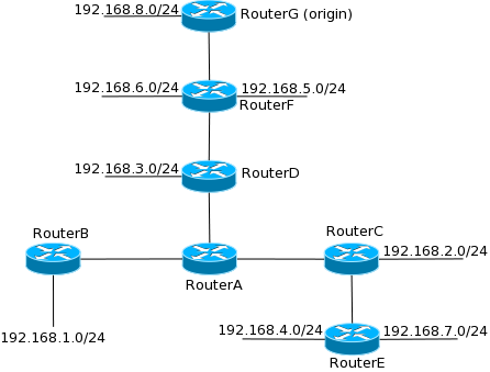
Once OSPF exchanges link state advertisements and populates the topology table, each router runs a calculation on the information collected. These calculations use something known as the Shortest Path First (SPF) algorithm. To do so, each router creates a tree putting itself at the root of the tree and the other routers and networks form the branch and leaves. In effect the router puts itself at the start and the area branches out from it. Figures 5-7 and 5-8 show an example of how the SPF tree is created by a router. Figure 5-7 shows the SPF tree with RouterA as the origin while Figure 5-8 shows the SPF tree with RouterG as the origin. Notice how different the network looks from the perspective of each router. The benefit of each router creating this tree is that the shortest path can be found from each router to each destination and there is no routing by rumor as seen with distance vector protocols.
Figure 5-7 SPF tree Example 1
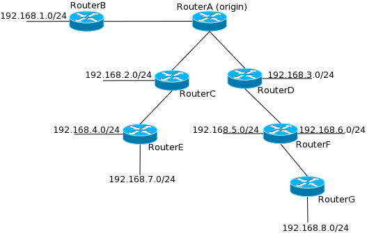
Figure 5-8 SPF tree Example 2
It is important to understand that each router creates this tree only for the area it belongs to. If a router belongs to multiple areas, it will create a separate tree for each area.
A big part of the tree is also the cost associated with each path. Cost is the metric used by OSPF is the sum of the cost of the entire path from the router to the remote network. The OSPF RFC defines cost as an arbitrary value, so Cisco calculates cost as 108/bandwidth. Bandwidth in this equation is the bandwidth configured on the interface. Using this equation, an Ethernet interface with a bandwidth of 10Mbps has a cost of 10 and a 100Mbps interface has a cost of 1. You may have noticed that interfaces having a bandwidth of more than 100Mbps will have a cost in fraction but Cisco does not use fractions and rounds of the value to 1 for such interfaces.
In Figure 5-8, if all interfaces are FastEthernet interfaces with a bandwidth of 100Mbps, each link has a cost of 1. So for the path from RouterG to the 192.168.7.0/24, the total cost will be 5 and to the network 192.168.3.0/24, the total cost will be 2.
The cost of each interface can be changed using the ip ospf cost command in the interface configuration mode. It should be noted that since the OSPF RFC does not exactly define the metric that makes up the cost, each vendor uses a different metric. When using OSPF in a multivendor environment, you will need to adjust cost to ensure parity.
Link State Advertisements
The fundamental building blocks of OSPF are the link state advertisements that are sent from every router to advertise links and their states. Given the complexity and scalability of OSPF, different LSA types are used to keep the OSPF database updated. Out of the various LSAs, the first five are most relevant to the limited OSPF discussion covered in this chapter and are discussed below:
- Type 1 – Router LSA – Each router in the area sends this LSA to announce its presence and list the links to other routers and networks along with metrics to them. These LSAs do not cross the boundary of an area.
- Type 2 – Network LSA – The DR in a multi-access network sends out this LSA. It contains a list of routers that are present in the network segment. These LSAs also do not cross the boundary of an area.
- Type 3 – Summary LSA – The ABR takes the information learned in one area (and optionally summarizes this information) and sends it out to another area it is attached to. This information is contained in LSA type 3 and is responsible for propagation of Inter-area routes.
- Type 4 – ASBR Summary LSA – ASBRs originate external routes (redistributed routes) and send them throughout the network. While the external routes are listed in type 5 LSA, the details of the ASBR themselves in listed in type 4 LSAs. This LSA is originated by the ABR of the area where the ASBR resides.
- Type 5 – External LSA – This LSA lists routes redistributed into OSPF from another OSPF process or another routing protocol. This LSA is originated by the ASBR and propagates across the OSPF AS.